The beginning

The other day I was asked by a colleague to prepare high-resolution figures using data from a project. She had prepared them by doing screenshots from a web interface, but not only the resolution was not good enough, the quality of the figure was not great.

In this post we will see how we can do something nicer with a few lines of code.

The idea

First of all: what do we want to get? According to the requirements:

• resolution about 300 dpi (or more) → easy!
• aspect ratio of the plot: 1.78 approx. → not difficult, but need fine-tuning
• something that looks nice, with data points located on a map.

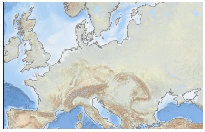
My idea was to use the EMODnet Bathymetry as the map background, so I directly have the depth and the coastline. Then on top of that, I will add the data points and the 2-dimensional field.

Instead of downloaded the bathymetry in netCDF, then plotting it with functions such as pcolor or contourf, I thought that WMS (Web Map Service) could make things easier. WMS is a protocol developed by the Open Geospatial Consortium and was designed to request geo-registered images from geospatial databases.

The EMODnet bathymetry server can be reached at http://ows.emodnet-bathymetry.eu/wms and the layers of interest are called ‘emodnet:mean_atlas_land’ and ‘coastlines’.

The tools: Basemap or Cartopy?

I’ve been writing about Basemap and Cartopy several times in this blog, for example here and here. Even after quite a long time using it, I still try things first with Basemap, though I know it is not developed anymore.
The thing is, when you need to update to something new (for example going from Python to Julia), there is always some kind of inertia, or simply a lack of time to spend on learning. Here there was a good reason to settle for Cartopy: I want to use add WMS layer, and with Basemap, it is not so straightforward.

First try with Basemap

The method is described in the Basemap doc, in summary the call looks like:

wmsimage(server, layers=[...], ...)

Using EMODnet Bathymetry WMS:

fig = plt.figure(figsize=(12, 8))
lonmin, lonmax, latmin, latmax = -10., 40., 40., 60.
m = Basemap(llcrnrlat=latmin, urcrnrlat=latmax, llcrnrlon=lonmin, urcrnrlon=lonmax, lat_ts=50, resolution='i', epsg=3857)
m.wmsimage('http://ows.emodnet-bathymetry.eu/wms?', layers=['emodnet:mean_atlas_land', 'coastlines'])
plt.show()

we get something that looks good. Note that we have to well specify the epsg parameter, otherwise we can end up with a blank plot without any error message.

So yes, it works with Basemap, now let’s check with Cartopy (I have to admit it did not work when I start drafting this post, but then I was able to find a solution).

Cartopy

I will provide more details here, as this is supposed to be the preferred solution. First, let’s define the projection, here we want to use Mercator.

import cartopy
import cartopy.crs as ccrs
import matplotlib.pyplot as plt

coordinates = [-31., 23., 46., 64]
myproj = ccrs.Mercator(central_longitude=0.5 * (coordinates[0] + coordinates[1]), min_latitude=coordinates[2], max_latitude=coordinates[3], globe=None, latitude_true_scale=None)

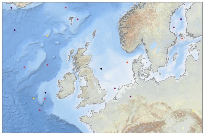
Then we create a set of fake data points, within our domain of interest:

import
dlon = coordinates[1] - coordinates[0]
dlat = coordinates[3] - coordinates[2]

NN = 20
lon = [coordinates[0] + random.random() * dlon for iii in range(0, NN)]
lat = [coordinates[2] + random.random() * dlat for iii in range(0, NN)]
field = [random.random() * dlat for iii in range(0, NN)]

Now we have all we need for a simple test:

fig = plt.figure(figsize=(12, 12))
ax = plt.axes(projection=myproj)
scat = ax.scatter(lon, lat, s=20, c=field, cmap=plt.cm.inferno_r,
                  transform=ccrs.PlateCarree())
ax.add_wms(wms='http://ows.emodnet-bathymetry.eu/wms',
               layers=['emodnet:mean_atlas_land', 'coastlines'],
               transform=myproj)
plt.show()

Yes it works! Now time to explain why it works.

• We specify which projection we want to use for the plot:
  ax = plt.axes(projection=myproj)
• We add a transform= optional arguments to the scatter function call. According to the doc, when the transform argument is not supplied, it means that the coordinate system matches the projection. If we try to remove transform=, we will get an error due to the coordinate change:

  ...
  ValueError: zero-size array to reduction operation maximum which has no identity
  

Another way to avoid the error would be to set the projection to PlateCarree:

data_crs = ccrs.PlateCarree()
fig = plt.figure(figsize=(12, 12))
ax = plt.axes(projection=data_crs)
scat = ax.scatter(lon, lat, s=20, c=field, cmap=plt.cm.inferno_r)
ax.add_wms(wms='http://ows.emodnet-bathymetry.eu/wms',
               layers=['emodnet:mean_atlas_land', 'coastlines'])
plt.show()

The points are located at the same locations as the previous figure, but obviously the aspect ratio of the figure is different because of the projection.

So basically, the key is to understand the transform= option: it has to be used to specify which projection is used for the object we want to plot, it can be the data or something else.

Making things nicer

At the end we want something nice and clean, which can easily be done by adding a few lines of code to the basic example. What about adding?

• a color bar?
• longitude and latitude labels?
• a grid? and even better, using real data?

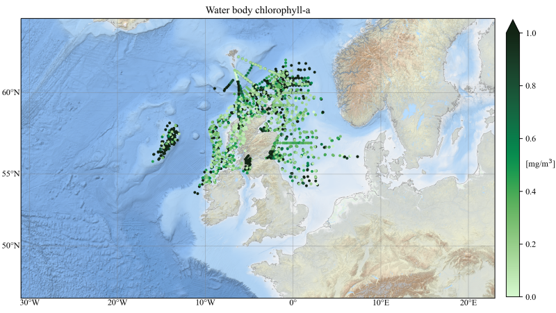
This is what had been done in this notebook, though I will add the code here for completeness:

import matplotlib.pyplot as plt
import cartopy
import cartopy.crs as ccrs
import netCDF4
import cmocean
import numpy as np
import cartopy.mpl.gridliner as gridliner
import matplotlib.ticker as mticker
import cartopy.mpl.ticker as cartopyticker

lon_formatter = cartopyticker.LongitudeFormatter()
lat_formatter = cartopyticker.LatitudeFormatter()
coordinates = [-31., 23., 46., 64]

fig = plt.figure(figsize=(12, 12))
ax = plt.subplot(111, projection=myproj)

scat = ax.scatter(lon2, lat2, s=5, c=field2,
                  vmin=0., vmax=1., cmap=cmocean.cm.algae,
                  transform=ccrs.PlateCarree())

cb = plt.colorbar(scat, extend="max", shrink=.5, pad=0.02)
cb.set_label("[mg/m$^3$]", rotation=0, ha="left", labelpad=-12.5)

ax.set_extent(coordinates)

ax.add_wms(wms='http://ows.emodnet-bathymetry.eu/wms',
               layers=['emodnet:mean_atlas_land', 'coastlines'],
               transform=myproj)

gl = ax.gridlines(crs=ccrs.PlateCarree(), draw_labels=True,
                  linewidth=.5, color='gray', alpha=0.5, linestyle='-')
gl.xlabels_top = False
gl.ylabels_right = False
gl.xlocator = mticker.FixedLocator(np.arange(-30., 21., 10.))
gl.ylocator = mticker.FixedLocator(np.arange(50, 61., 5.))

plt.title("Water body chlorophyll-a")
plt.show()