If you have ever been running (a lot) in the same town or village, you might want to know if you have covered most of the streets and trails. In this post we will see how to create a map summarizing all the information.

Getting the data

The plan is to get all the tracks from the platform you are using with your device. Here we work with Movescount (Suunto). Until recently, one could easily request all the moves using the export option, available in the Settings: https://www.movescount.com/settings#export

Usually the data arrives pretty fast, a few minutes later. What do we get? An archived containing a folder Moves, in which we have all the moves recorded with the device (more than 2500 in my case).

Update

Due to change in Suunto move management, I had to switch to a more manual method. The log files are not directly extracted from the watch using the openambit project.

It is quite strange to have to rely on code not written by Suunto, but hey, if they cannot ensure the data transfer, then the watch is kind of useless.

Data preparation

Converting to GPX

.fit files

When you export from Movescount, the file format is .fit. It can easily be converted to .gpx using the awesome gpsbabel tool. The command for the conversion reads:

gpsbabel -i garmin_fit -f input.fit -o gpx -F output.gpx

and we can loop on all the files to apply this conversion.

.log files

If you use Openambit, you end up with .log files that you can convert to gpx using a tool provided with Openambit: openambit2gpx.py. The file name is quite explicit.

Selection by type of activity

Movescount

When downloaded from Movescount, the type of activity (Running, Walking, Trekking) is written in the file name, so the job is already done.

We can remove static activities, such as Stretching, Indoor_training, in which there is no displacement.

Openambit

With Openambit, we don’t have access to the activity type. It might be necessary to implement a way to detect it from the total distance, the mean speed, or any other combination of relevant metrics.

This might be a good application of Machine Learning techniques, since we already have a ready training set.

Selection by region

If you have traveled and run in different places, it could be useful to classify the track by region. How to do that? Probably there are many ways, using for example geo-referencing. What we did is to base the classification on the distance between

• the average position of a track (mean longitude and latitude) and
• a coordinate representative of a region or town, it can be its center for example. If that computed distance is below a given threshold, then the track becomes to that region.

Of course we could use a geocoder such as geopy, though here we prefered to keep it simple.

Example

For Vienna, we consider the tracks for which the distance to the point (48.20467°N, 16.343028°E) is lower than 12 km. The threshold distance depends on the extension of the region.

In another example, we want to have all the tracks located in Mallorca island: the distance is computed from (39.624293°N, 3.025380°E), with a threshold of 60 km.

Results

Files

After all this we end up with GPX files classified by region. It is then straightforward to read the coordinates from the files and generate plots.

Figures

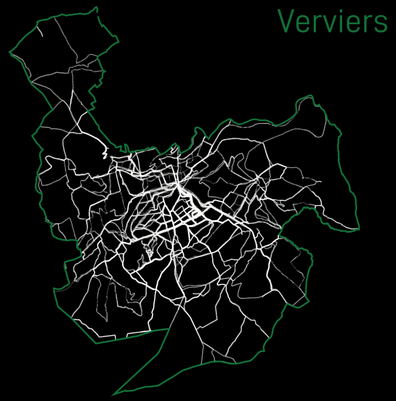
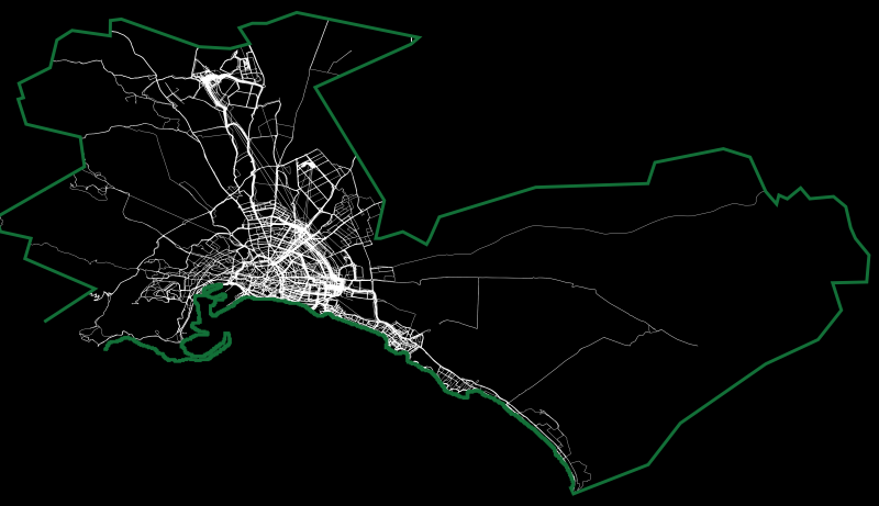
There are many types of visualisation to be done: simple lines, heatmaps, hexbin maps, radial plots… Here we just show an example with the running sessions in Verviers from 2017 to 2020.