Making plot with Cartopy and Julia
04 September 2019
Julia, Cartopy, PyPlot
Oceanography, Maps
A quick example of how to work with Cartopy and Julia to process and visualise 2D fields and visible images.
using NCDatasets
using PyPlot
using ImageView
using ArchGDAL
using PyCall
using Conda
Conda.add("cmocean")
Data
We will use:
- Sentinel-2 image (geoTIFF format) downloaded from the Sentinel-Hub browser and
- A netCDF file containg measurements of chlorophyll concentration, also Sentinel-2.
imagefile = "/data/Visible/Sentinel-2_L2A_2019-08-09c.tiff"
datafile = "/data/Sentinel2/S2A_MSI_2019_08_09_10_00_31_T34VCK_L2W.nc"
isfile(imagefile) & isfile(datafile)
true
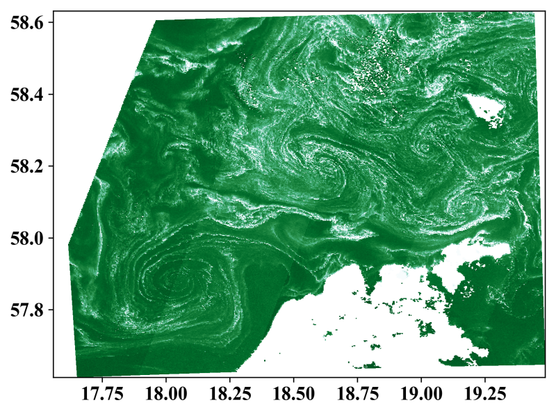
Reading the netCDF file
That’s an easy job if we use the NCDatasets module.
function read_chloro(datafile::String)
    local lon, lat, chl_oc3
    NCDatasets.Dataset(datafile, "r") do ds
        lon = ds["lon"][:]
        lat = ds["lat"][:]
        chl_oc3 = ds["chl_oc3"][:]
    end
    return lon, lat, chl_oc3
end
read_chloro (generic function with 1 method)
lon, lat, chl_oc3 = read_chloro(datafile);
Let’s make a quick plot:
NN = 20
PyPlot.pcolormesh(lon[1:NN:end,1:NN:end], lat[1:NN:end,1:NN:end],
    chl_oc3[1:NN:end,1:NN:end], cmap=PyPlot.cm.BuGn_r,
    vmin=0.95, vmax=7.5)
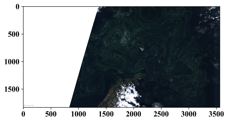
Reading the geoTIFF
We will use the ArchGDAL package to access the information from the geoTIFF file.
The function below reads the dimensions, the coordinates and the 2D layer.
function read_geotiff(filename::String)
    local field, lon, lat, proj4, extent
    ArchGDAL.registerdrivers() do
        ArchGDAL.read(filename) do dataset
            width = ArchGDAL.width(dataset)
            height = ArchGDAL.height(dataset)
            field = ArchGDAL.read(dataset)
            gt = ArchGDAL.getgeotransform(dataset)
            dx, dy = gt[2], -gt[end]
            x0 = gt[1] + dx/2
            x1 = x0 + (width-1) * dx
            y1 = gt[4] - dy/2
            y0 = y1 - (height-1)*dy

            proj4 = strip(ArchGDAL.toPROJ4(ArchGDAL.importWKT(ArchGDAL.getproj(dataset))))
            lon = x0:dx:x1
            lat = y0:dy:y1

            extent = (x0, x1, y0, y1)
        end
    end
    return lon, lat, field, proj4, extent
end
read_geotiff (generic function with 1 method)
lonvis, latvis, imagevis, proj4, extent = read_geotiff(imagefile);
@info("Image size: $(size(imagevis))")
┌ Info: Image size: (3564, 1833, 3)
└ @ Main In[4]:2
For the plot we can simply use the imshow() method.
Note the permutation applied to the first 2 dimensions of the field.
PyPlot.imshow(permutedims(imagevis, (2,1,3)))
Plotting with Cartopy
The installation of Cartopy with Julia is not explained in details here. A solution is to use the Conda module and then install Cartopy with:
using Conda
Conda.add("Cartopy")
Cartopy is a Python module hence it is not directly imported by Julia.
ccrs = pyimport("cartopy.crs")
PyObject <module 'cartopy.crs' from '/home/ctroupin/.julia/conda/3/lib/python3.7/site-packages/cartopy/crs.py'>
Create a projection
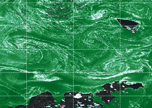
We will use a Plate-Carrée projection.
myproj = ccrs.PlateCarree();
Make the plot
Just combining the different elements and limiting the domain to the chlorophyll field:
PyPlot.figure(figsize=(8, 8))
ax = PyPlot.subplot(111, projection=myproj)
ax.pcolormesh(lon, lat, chl_oc3, cmap=PyPlot.cm.BuGn_r,
    vmin=0.95, vmax=7.5)
PyPlot.imshow(permutedims(imagevis, (2,1,3)), extent=extent)
ax.set_xlim(minimum(lon), maximum(lon))
ax.set_ylim(minimum(lat), maximum(lat))
gl = ax.gridlines(crs=myproj, linewidth=.5, color="white",
    alpha=0.9, linestyle="--", zorder=6)
PyPlot.savefig("./visible_chloro_julia.png", dpi=300, bbox_inches="tight")
Final remarks
- I’m quite new to
Cartopyso there are probably many ways to improve the figure. - For the final plot you may want to use the full resolution for the 2D field (i.e. setting NN=1). Just take into account that this may take a while, more than 20 minutes in my case, with the computer almost not responding.
- The
PyPlot.prefixes of the commands can certainly be removed, but I prefer to keep them for explicitness.