Reading and displaying geoTIFF images with Python
30 August 2019
Python, Basemap, Cartopy
Oceanography, Maps
In this post we explain how to add a visible image as a background for a map.
The geoTIFF files used in this example are taken from the Sentinel-Hub browser or from the NASA WorldView.
Note that you be logged in if you want to export the image in geoTIFF format from Sentinel Hub.
import os
from mpl_toolkits.basemap import Basemap
import matplotlib.pyplot as plt
import numpy as np
import matplotlib.colors as colors
from osgeo import gdal
from osgeo import osr
import tempfile
import subprocess
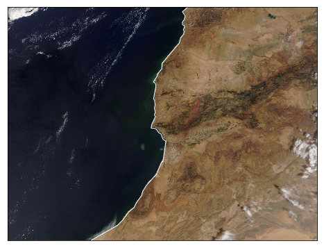
datafile1 = "/data/Visible/MODIS-Terra-20160913.tiff"
datafile2 = "/data/Visible/Sentinel-2_L2A_2019-08-09.tiff"
1. Reading the geoTIFF
ds = gdal.Open(datafile1, gdal.GA_ReadOnly)
ds.GetProjectionRef()

# Read the array and the transformation
arr = ds.ReadAsArray()
# Read the geo transform
trans = ds.GetGeoTransform()
# Compute the spatial extent
extent1 = (trans[0], trans[0] + ds.RasterXSize*trans[1],
          trans[3] + ds.RasterYSize*trans[5], trans[3])

# Get the info on the projection
proj = ds.GetProjection()
inproj = osr.SpatialReference()
inproj.ImportFromWkt(proj)
print(inproj)

# Compute the coordinates
x = np.arange(0, ds.RasterXSize)
y = np.arange(0, ds.RasterYSize)

xx, yy = np.meshgrid(x, y)
lon1 = trans[1] * xx + trans[2] * yy + trans[0]
lat1 = trans[4] * xx + trans[5] * yy + trans[3]

# Transpose
arr1 = np.transpose(arr, (1, 2, 0))
GEOGCS["WGS 84",
    DATUM["WGS_1984",
        SPHEROID["WGS 84",6378137,298.257223563,
            AUTHORITY["EPSG","7030"]],
        AUTHORITY["EPSG","6326"]],
    PRIMEM["Greenwich",0],
    UNIT["degree",0.0174532925199433],
    AUTHORITY["EPSG","4326"]]
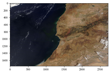
Here we don’t have to modify the longitude and latitude as they are already in degrees.
Note that the array dimensions are permuted, this is because we want to use it with imshow() function.
We’ll explain in more details how to make nice plots.
plt.imshow(arr1)
plt.show()
Let’s put all that in a function and apply it to another image from Sentinel-Hub.
def read_geotiff(imagefile):
    """
    Read an image and compute the coordinates from a geoTIFF file
    """
    ds = gdal.Open(imagefile, gdal.GA_ReadOnly)
    ds.GetProjectionRef()

    # Read the array and the transformation
    arr = ds.ReadAsArray()
    # Read the geo transform
    trans = ds.GetGeoTransform()
    # Compute the spatial extent
    extent = (trans[0], trans[0] + ds.RasterXSize*trans[1],
              trans[3] + ds.RasterYSize*trans[5], trans[3])

    # Get the info on the projection
    proj = ds.GetProjection()
    inproj = osr.SpatialReference()
    inproj.ImportFromWkt(proj)

    # Compute the coordinates
    x = np.arange(0, ds.RasterXSize)
    y = np.arange(0, ds.RasterYSize)

    xx, yy = np.meshgrid(x, y)
    lon = trans[1] * xx + trans[2] * yy + trans[0]
    lat = trans[4] * xx + trans[5] * yy + trans[3]

    # Transpose
    arr = np.transpose(arr, (1, 2, 0))

    return lon, lat, arr, inproj, extent
lon2, lat2, arr2, inproj2, extent2 = read_geotiff(datafile2)
Let’s have a look on the projection information:
print(inproj2)
PROJCS["WGS 84 / Pseudo-Mercator",
    GEOGCS["WGS 84",
        DATUM["unknown",
            SPHEROID["unnamed",6378137,0,
                AUTHORITY["EPSG","1"]],
            AUTHORITY["EPSG","1"]],
        PRIMEM["Greenwich",0],
        UNIT["degree",0.0174532925199433],
        AUTHORITY["EPSG","4326"]],
    PROJECTION["Mercator_1SP"],
    PARAMETER["central_meridian",0],
    PARAMETER["scale_factor",1],
    PARAMETER["false_easting",0],
    PARAMETER["false_northing",0],
    UNIT["metre",1,
        AUTHORITY["EPSG","9001"]],
    EXTENSION["PROJ4","+proj=merc +a=6378137 +b=6378137 +lat_ts=0.0 +lon_0=0.0 +x_0=0.0 +y_0=0 +k=1.0 +units=m +nadgrids=@null +wktext  +no_defs"],
    AUTHORITY["EPSG","3857"]]
Without going into details, we see that we are not working with degrees and that a transformation has to be performed.
We will use the tool gdalwarp to do that but I’m sure it can be done in native Python.
The command to looks like:
gdalwarp input.tiff output.tiff -t_srs "+proj=longlat +ellps=WGS84"
This creates a new geoTIFF file where the coordinates are using the World Geodetic System 1984.
Now let’s introduce that in the reading function. We will create a temporary file as the output of the command, keeping the input file unchanged, and apply the same reading steps to the temporary file.
def read_geotiff(imagefile):
    """
    Read an image and compute the coordinates from a geoTIFF file
    """

    # Create temporaty file
    fd, path = tempfile.mkstemp()

    # Prepate the command (bash)
    command = 'gdalwarp {} {} -t_srs "+proj=longlat +ellps=WGS84"'.format(imagefile, path)
    print(command)
    subprocess.run(command, cwd=os.path.dirname(imagefile),
                   stdout=subprocess.PIPE, shell=True)

    ds = gdal.Open(path, gdal.GA_ReadOnly)
    ds.GetProjectionRef()

    # Read the array and the transformation
    arr = ds.ReadAsArray()
    # Read the geo transform
    trans = ds.GetGeoTransform()
    # Compute the spatial extent
    extent = (trans[0], trans[0] + ds.RasterXSize*trans[1],
              trans[3] + ds.RasterYSize*trans[5], trans[3])

    # Get the info on the projection
    proj = ds.GetProjection()
    inproj = osr.SpatialReference()
    inproj.ImportFromWkt(proj)

    # Compute the coordinates
    x = np.arange(0, ds.RasterXSize)
    y = np.arange(0, ds.RasterYSize)

    xx, yy = np.meshgrid(x, y)
    lon = trans[1] * xx + trans[2] * yy + trans[0]
    lat = trans[4] * xx + trans[5] * yy + trans[3]

    # Transpose
    arr = np.transpose(arr, (1, 2, 0))

    return lon, lat, arr, inproj, extent
lon2, lat2, arr2, inproj2, extent2 = read_geotiff(datafile2)
gdalwarp /data/Visible/Sentinel-2_L2A_2019-08-09.tiff /tmp/tmpsrjih4w6 -t_srs "+proj=longlat +ellps=WGS84"
Let’s check again the projection info:
print(inproj2)
GEOGCS["WGS 84",
    DATUM["unknown",
        SPHEROID["WGS84",6378137,298.257223563]],
    PRIMEM["Greenwich",0],
    UNIT["degree",0.0174532925199433]]
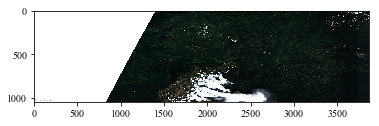
and we can have a quick check with imshow():
plt.imshow(arr2)
plt.show()
2. Plotting the image
2.1 Matplotlib only
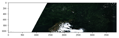
The first method is what we showed in the previous cells: using imshow(). The problem is that you cannot use the coordinates directly.
plt.figure(figsize=(8, 8))
plt.imshow(arr2)
plt.show()
2.2 With Basemap
We start by creating a Mercator projection in the region of interest.
m = Basemap(projection='merc',
        llcrnrlon=lon1.min(), llcrnrlat=lat1.min(),
        urcrnrlon=lon1.max(), urcrnrlat=lat1.max(),
        lat_ts= 0.5 * (lat1.min() + lat1.max()), resolution="i")
Now let’s plot the image and add the coastline on it to ensure they are aligned.
plt.figure(figsize=(8, 8))
m.imshow(arr1)
m.drawcoastlines(linewidth=1, color="w")
plt.show()
plt.close()
Obviously we have a small issue, the visible image is upside-down, that is solved in a few seconds.
plt.figure(figsize=(8, 8))
m.imshow(np.flipud(arr1))
m.drawcoastlines(linewidth=1, color="w")
plt.show()
plt.close()
the results now seems correct, at least visually.
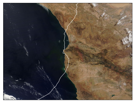
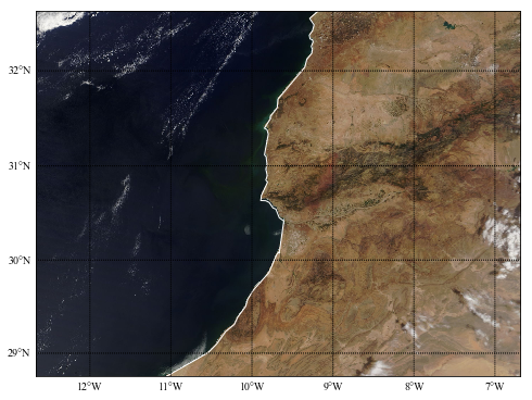
We can add more features to the map: labels, meridians, etc.
plt.figure(figsize=(8, 8))
m.imshow(np.flipud(arr1))
m.drawcoastlines(linewidth=1, color="w")
m.drawmeridians(np.arange(-12., -5., 1), labels=(0,0,0,1))
m.drawparallels(np.arange(25., 35., 1.), labels=(1,0,0,0))
plt.show()
plt.close()
2.3 With Cartopy
Since Basemap is deprecated in favor of the Cartopy project, it is relevant to show how to make this plots with Cartopy. We use this example to guide us.
import cartopy
import cartopy.crs as ccrs
We start with the plate carrée projection:
myproj = ccrs.PlateCarree()
plt.figure(figsize=(8, 8))
ax = plt.axes(projection=myproj)
ax.imshow(arr1, origin='upper', extent=extent1, transform=myproj)
ax.coastlines(resolution='10m', color="red")
plt.show()
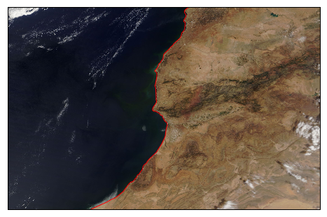
the results is correct, now let’s try another projection, Mercator:
myproj = ccrs.Mercator()
plt.figure(figsize=(8, 8))
ax = plt.axes(projection=myproj)
ax.imshow(arr1, origin='upper', extent=extent1)
ax.coastlines(resolution='110m', color="red")
plt.show()
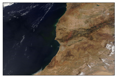
Something is wrong here: the coastline does not appear.
It seems that only the plate carrée works for the case.